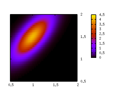
#
# Suppose we have two measured values, X and Y, with statistical errors
# of 10 %. This measured quantities also have a common systematic error
# of 0.2 (absolute error). The probability density function can be expressed
# by a bivariate Gaussian distribution which has a center value of X and Y
# with variances of 0.1*X+0.2 and 0.1*Y+0.2, respectively.
#

# Measured values for quantities X and Y
mx = 1.0
my = 1.5

# Uncertainties in measured X and Y (both 10%)
sigx = 0.1 * mx
sigy = 0.1 * my

# Common error
sc = 0.2

# Total errors
sx = sqrt(sigx*sigx + sc*sc)
sy = sqrt(sigy*sigy + sc*sc)

# Correlation
c = sc*sc/sx/sy

g(x,m,s) = (x-m)/s
f(x,y,c) = exp(-1/(2*sqrt(1-c*c))*\
(  g(x,mx,sx)**2\
-2*c*g(x,mx,sx)*g(y,my,sy)\
+g(y,my,sy)**2))/(2*pi*sx*sy*sqrt(1-c*c))

unset surface
set view 0,0
set format z ""
unset ztics
set isosample 40,40
set size square
set xrange [0.5:2]
set yrange [0.5:2]
set xtics 0.5
set ytics 0.5
set pm3d

splot f(x,y,c)