- not so Frequently Asked Questions -
update 2004/9/16
|
|
- not so Frequently Asked Questions - update 2004/9/16
|
|
not so FAQ |
Miscellaneous Stuff (No.2)Least-Squares Fitting with non-linear functions (I)Gnuplot3.7 has a provision of a least-squares fitting. It searches automatically for parameters of an arbitrary function by fitting it to data in a file. The function can be linear or non-linear, but it should be expressed by gnuplot's expression manner. Here is an example for data fitting -- fit a Lorentzian function f(x)=a/(1+b*x*x) to data. The variables a and b are the parameters. The following sample data were prepared by calculating this function with a=2 and b=1, to show that gnuplot gives the correct answer. -10.000000 0.019802 -8.947370 0.024674 -7.894740 0.031582 -6.842110 0.041828 -5.789470 0.057941 -4.736840 0.085333 -3.684210 0.137236 -2.631580 0.252359 -1.578950 0.572561 -0.526316 1.566160 0.526316 1.566160 1.578950 0.572561 2.631580 0.252359 3.684210 0.137236 4.736840 0.085333 5.789470 0.057941 6.842110 0.041828 7.894740 0.031582 8.947370 0.024674 10.000000 0.019802 Those numerical data are stored into the data-file "exp.dat". Firstly the fitting function is defined. The parameters to be searched for are arbitrary except for "x" or "t" those gnuplot uses. A data fitting begins by the command fit . The parameter names are given by the via option. At the data fitting, one can use using, index, every options to specify or to skip data or data block in the file. An uncertainty of the data point is treated as a weight of it. When the data point has an error of sigma, the weigh becomes sigma^{-2}. To do the weighted least-squares fitting, the errors are prepared at the third column in your data-file, then you have to tell that those are the uncertainties, like fit f(x) "exp.dat" using 1:2:3 via a,b . When the data error is omitted, all data points have the equivalent weight. gnuplot> f(x)=a/(1+b*x*x) gnuplot> fit f(x) "exp.dat" via a,b Iteration 0 WSSR : 1.43879 delta(WSSR)/WSSR : 0 delta(WSSR) : 0 limit for stopping : 1e-05 lambda : 0.201184 ....... Final set of parameters Asymptotic Standard Error ======================= ========================== a = 2 +/- 5.236e-07 (2.618e-05%) b = 0.999998 +/- 7.397e-07 (7.397e-05%) correlation matrix of the fit parameters: a b a 1.000 b 0.837 1.000 During the data fitting, you can see changes in the parameters on your display. The same stuff you can find in a file "fit.log" which is generated in the current directory. If succeeded, you get the final values of the parameter as well as those covariance matrix. In the above case, the correct parameters a=2 and b=1 were obtained. The final results are stored in the variables, a and b, so that you can compare the fitted function and the data by plotting this function with the fitted parameters. gnuplot> plot f(x) with lines, "exp.dat" using 1:2 w points 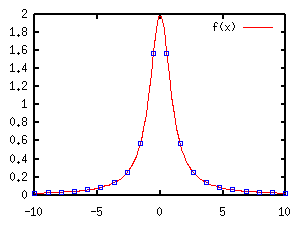  Least-Squares Fitting with non-linear functions (II)The next example is more realistic one. We have experimental data like below. A function f(x)=c*(x-a)**b is fitted to the data by adjusting the variables a, b, and c. # X Y Z 6.295 8.4 0.3 6.795 23.9 0.7 7.826 104.0 3.0 8.830 255.0 8.0 9.841 421.0 13.0 10.860 566.0 18.0 11.864 690.0 22.0 Each data point has an error (Z), then the weight of the point is 1/Z*Z. At first, plot the experimental data only to see their tendency. gnuplot> set log y gnuplot> plot "exp.dat" using 1:2:3 w yerrorbars 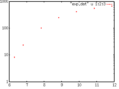 Next, choose initial values of those variables, a, b, and c. When the initial values are not given at the parameter search, gnuplot assumes that those values are 1. Since this choice is insufficient in some case, you should give better initial values. Our fitting function is f(x)=c*(x-a)**b, then one can guess that a is near 6 because f(x)=0 at x=a, c is in the order of 10 (see log(f(x))), and b is 1 or 2 as f(x) becomes 10 to 100 times when x is increased by 1. Those values are used for the initial. gnuplot> a=6 gnuplot> b=1 gnuplot> c=10 gnuplot> f(x)=c*(x-a)**b gnuplot> fit f(x) "exp.dat" using 1:2:3 via a,b,c The calculation converges after 17 times iteration, the final values with those covariance are displayed. The values obtained were a=5.77, b=1.89, c=25.8. After 17 iterations the fit converged. final sum of squares of residuals : 90.8196 rel. change during last iteration : -9.71916e-09 degrees of freedom (ndf) : 4 rms of residuals (stdfit) = sqrt(WSSR/ndf) : 4.76497 variance of residuals (reduced chisquare) = WSSR/ndf : 22.7049 Final set of parameters Asymptotic Standard Error ======================= ========================== a = 5.76731 +/- 0.176 (3.051%) b = 1.89369 +/- 0.2127 (11.23%) c = 25.7956 +/- 9.807 (38.02%) correlation matrix of the fit parameters: a b c a 1.000 b -0.944 1.000 c 0.975 -0.975 1.000 Those results were compared with the experimental data. gnuplot> plot f(x),"exp.dat" using 1:2:3 w yerrorbars 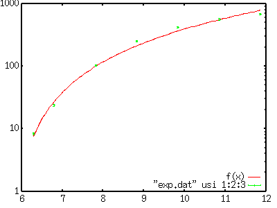 |