About 2-Dimensional Plot (No.2)

I want to draw a zero axis.

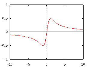
use set {x|y}zeroaxis command. If no option is provided, the zero-axis line is drawn by line-type 0 (dotted line). The options ls line_style, lt line_type, lw line_width control the style of the zero axis. In the case of lt -1 , the line becomes the same as the border lines.

gnuplot> set xzeroaxis lt -1
gnuplot> set yzeroaxis

I want to get rid of small bars which appear at the top of error bars.

Small bars are placed on the top (bottom) of the error bars when data with the errors are plotted. This lines are sometimes bothersome when the number of data is large. To get rid of them :

gnuplot> set bar 0

The option is the length (default 1) of the bar. If 0, the bar disappears.

Note that even if you change the size of points by set pointsize, the length of this bar does not change. You'd better to change the bar size at the same time.

gnuplot> set pointsize 3
gnuplot> set bar 3

I want to make letters larger.

It depends on the devices with which you are plotting the figure. Commands of set label or set title accept a font option, so you can use the larger fonts if those are provided for the device. But it is usually difficult to control the size of fonts.

If you are using the postscript terminal, scaling of the font is easy. Instead of enlarging the letters, make the whole figure smaller. Then the font size becomes large relative to the figure size. It is possible to resize the PostScript figure, so that it is no problem even if your figure is too small.

gnuplot> set size 0.3,0.3

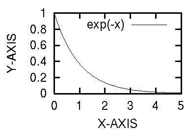
With the command above the whole size is reduced to 30 %. An Encapsulated PostScript terminal is used, and the figure is enlarged again at printing. This case is rather extreme, but the reduction in the size of 0.5 -- 0.7 yields a sufficient result.

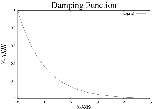
If you want to control the font precisely in your PostScript figure, use the font options of label, title, and specify the font-shape and its size. An option for the set terminal command also has a default font size option. In the following example, we used 16pt Helvetica for the basic font, and the title and axis names are shown by the different fonts.

gnuplot> set terminal postscript enhanced "Helvetica" 16
gnuplot> set title "Damping Function" font "Times-Roman,40"
gnuplot> set xlabel "X-AXIS" font "Helvetica,20"
gnuplot> set ylabel "Y-AXIS" font "Times-Italic,32"
gnuplot> plot exp(-x)

Well, it can be done as shown above, but I don't think it is convenient. Although gnuplot generates a nice figure, you can decorate your figures with other tools like Tgif.

I want to connect all points with some smooth curves.

Gnuplot has a provision for data smoothing with the cubic-splines or the Bezier curves. To display the smoothed curve, use the smooth option in the plot command. There is a difference between those smoothing methods. The spline function is an interpolation between the data points, while the Bezier curve is an approximation of the data trend.

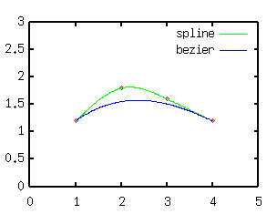
The following example is a comparison of the spline function and the Bezier curves. The same data are plotted in the three ways, the original data which are shown by the symbols, the curve smoothly interpolated with the spline function, and the Bezier curve.

gnuplot> plot "test.dat" using 1:2 notitle with points, \
>             "test.dat" using 1:2 smooth csplines \
>                                  title "spline" with lines,\
>             "test.dat" using 1:2 smooth bezier \
>                                  title "bezier" with lines

The spline option csplines connects all data points smoothly. On the other hand the Bezier curve is not an interpolation but it smoothes the data. The spline function can also be used for the data smoothing by the option acsplines , with which one can draw an approximation curve of the data. The example above the X and Y data are only needed, but to make an approximation curve one needs weights (uncertainties) of all data points. The next example shows how to smooth experimental data with the Bezier curve and the spline function.

gnuplot> plot "test.dat" using 1:2:3 notitle with yerrorbars, \
>             "test.dat" using 1:2:3 smooth acsplines \
>                                    title "acsplines" with lines,\
>             "test.dat" using 1:2   smooth bezier \
>                                    title "bezier"    with lines

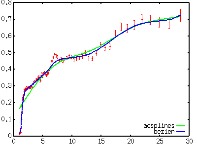
The Bezier curve chases the variation of the data, but the spline function expresses a rough trend of them. Sometimes one needs to draw a curve by "eye guide" in the plot of experimental data. Gnuplot can do it very easily.

The weights of the data are needed to make the approximation curve with the spline. If the weights are the same for all the data points, you can give an equal weight 1.0 by using 1:2:(1.0) .

I want to erase points those are on border.

Data points or lines near the border line can be clipped. The command set clip controls the method of this data clip. There are three types of the data clip, points , one , and two . In order to explain the difference of those types, the following example is used.

#  X     Y
1.0   1.0
2.0   1.5
3.0   2.0
4.0   1.5
5.0   1.0

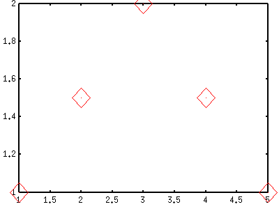
As the default, the first data point (X=1) and the last one (X=4) locate at the corners of the graph, and the mid point (X=3) is placed on the top border line. In the next example, data points are magnified by set pointsize 10 command to see clearly.

gnuplot> set pointsize 10
gnuplot> plot "test.dat" notitle with points

When the clip is defined the points on the border (X=1, 3, and 4) disappear.

gnuplot> set clip points
gnuplot> plot "test.dat" notitle with points

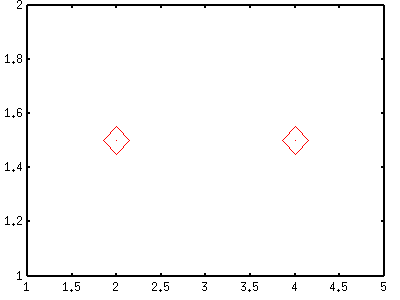
By the way gnuplot clips data automatically if those are very close to the border lines. For example, even if the Y range in the above figure is enlarged to 2.1, the data point at X=3 is still clipped. I don't know the criteria of this --- which point is clipped and which is shown.

The next clip type is set clip one , which defines a behavior of lines near the border. When there are two points, one is inside the graph and the other is outside, and if those two points are connected by a line which crosses the border line, there are two choices to control this. The first one is to draw a line from the inside point to the border line and truncate the line there. This is the default. Alternatively such lines can be erased by set noclip .

When a function is displayed, gnuplot calculates the X,Y values at certain points which are defined by sampling rate (100, default), and those points are connected by small lines. So that gnuplot draws truncated-lines instead of a curve. If some point is outside the graph, the line crosses the border line. The command set clip one specifies that the line is erased (noclip), or that the line is partly drawn from the end point to the border line (clip).

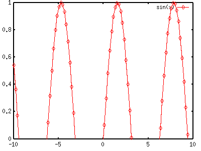
When the function y=sin(x) is drawn in a figure and the Y range is [0:1], the curve crosses the X axis several times. The function is displayed by with linespoints , then the points shown by a symbol are those gnuplot actually calculated.

gnuplot> set clip one
gnuplot> plot sin(x) with linespoints
gnuplot> set noclip one
gnuplot> replot

clip one

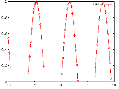noclip one

The last type of the clip is set clip two . This also controls when a truncated-line crosses the border line, but this is the case for that the both points are outside the graph. The default is clip . See the following example.

gnuplot> set yrange [-0.5:0.5]
gnuplot> set samples 10
gnuplot> set clip two
gnuplot> plot sin(x) with linespoints
gnuplot> set noclip two
gnuplot> replot

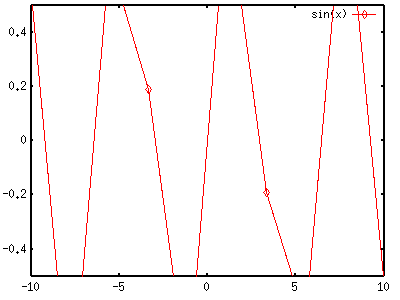clip two

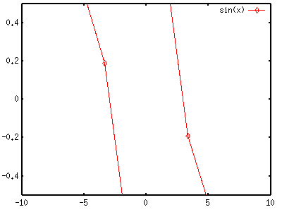noclip two